Kina Robotics

The simple robotic arm that is still interesting is a 3-DOF planar manipulator.

With just three revolute joints, it already exposes reach limits, redundancy trade-offs, and workspace structure. It is simple enough to model from scratch, yet reach enough to surface real design questions.

In this note, I’ll build the model from first principle and explore what its geometry tells us, not just how to compute positions, but what design choices actually change.

What Forward Kinematics Really Is

Forward kinematics (FK) answers a simple question:

Given the joint angles, where is the end-effector?

For deeper mathematical treatment,Forward Kinematics in 5 Easy Steps by Alex Owen-Hill, and Modeling, Motion Planning, and Control of Manipulators and Mobile Robots book are excellent references. But here, I’ll derive it directly from geometry.

We’ll consider a planar arm with 3 revolute joints:

• Joint angles: $\theta_1, \theta_2, \theta_3$
• Link lengths: $L_1, L_2, L_3$

All motion lies in the plane.

Each joint rotates relative to the previous link. So the orientation of each link accumulates:

• Link 1 orientation: $\theta_1$
• Link 2 orientation: $\theta_1 + \theta_2$
• Link 3 orientation: $\theta_1 + \theta_2 + \theta_3$

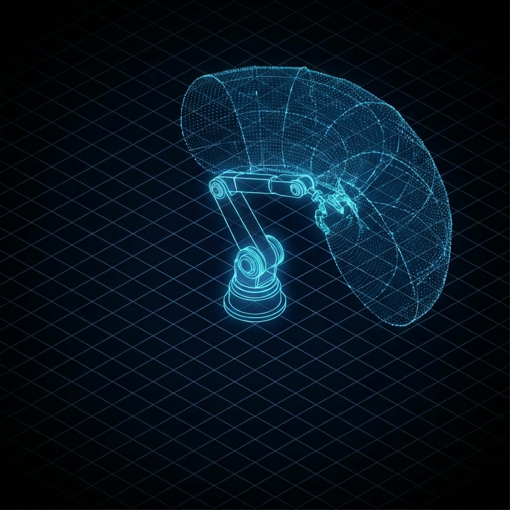
A visualization of this robot is shown below:

We can compute the position of the end-effector using the equations:

Notice that the second link’s position accumulates the rotation of the first and the third accumulates the rotation of the first two. This simple dependency is where most of the structure comes from.

This is the entire forward kinematics model:

import numpy as np
class Planar3R:
    """
    3-DOF planar RRR robot model.
    """
    def __init__(self, link_lengths, joint_limits=None):
        self.link_lengths = np.array(link_lengths)
        self.dof = 3
        if joint_limits is None:
            self.joint_limits = np.array([
                [-np.pi, np.pi],
                [-np.pi, np.pi],
                [-np.pi, np.pi]
            ])
        else:
            self.joint_limits = np.array(joint_limits)
    def forward_kinematics(self, q):
        """
        Compute end-effector (x, y) position.
        Parameters:
            q : iterable of 3 joint angles [rad]
        Returns:
            np.array([x, y])
        """
        L1, L2, L3 = self.link_lengths
        t1, t2, t3 = q
        x = (
            L1 * np.cos(t1) + L2 * np.cos(t1 + t2) + L3 * np.cos(t1 + t2 + t3)
        )
        y = (
            L1 * np.sin(t1) + L2 * np.sin(t1 + t2) + L3 * np.sin(t1 + t2 + t3)
        )
        return np.array([x, y])

What the Geometry Implies

The Maximum Reach

The Inner Unreachable Region

If one link is too long relative to the others, a “hole” appears in the center of the workspace. For example if:

Then there is a region in the base that is unreachable. The image below show the robot workspace with L1 = 1.5, L2, = 1, and L3 = 0.2.

Redundancy Trade-off

In 2D, a task space position (x,y) has two variable. But we have three joint angles. That means the system is redundant for positioning. For most reachable points, there are infinitely many joint solutions. This is powerful:

• You can avoid joint limits
• You can avoid obstacles
• You can minimize energy
• You can shape manipulability

But it also introduces decision-making because the robot must choose which possibility to use.

Singularities Are Visible in the Equations

Consider when the arm is fully stretched:

The links align. Small changes in joint angles produce very little change in lateral motion. This creates velocity collapse in certain directions.

Design Choices: What Actually Changes?

Now let’s ask a deeper question:

If I change link lengths, what fundamentally changes?

Increasing $L_1$ (the base link)

• Expands outer reach
• Increases swept area
• Amplifies distal inertia
• Enlarges singular region when extended

This is why long proximal links make robots powerful but heavy and dynamically expensive.

Increasing $L_3$ (the distal link)

• Increases fine positioning range
• Increases tip inertia significantly
• Makes precision harder in high speed motion

This is why distal links are often short and lightweight in industrial robots.

Making Links Equal Length

When:

The workspace becomes more uniform, manipulability distribution improves, and the arm becomes “balanced” geometrically. But this is rarely optimal for a specific industrial task. Task geometry often dictates asymmetry.

Configuration Space vs Workspace

When you sample uniformly in joint space (also called configuration space) and then you map those samples through forward kinematics:

this mapping is nonlinear, distorting volume. Some regions will look dense and some are sparse as shown in the image below. Here, the link lengths are [1.0, 1.0, 0.2] and the joint limits are $\theta_1=[-\pi/2, \pi/2]$, $\theta_2=[-\pi/2, \pi/2]$ and $\theta_3=[-\pi/2, \pi/2]$.

Here are the functions that uniformly samples the joint space:

    def sample_joint_space(self, n_samples):
        qs = []
        for i in range(self.dof):
            low, high = self.joint_limits[i]
            qs.append(np.random.uniform(low, high, n_samples))
        return np.vstack(qs).T

    def compute_workspace(robot, n_samples=10000):
    q_samples = robot.sample_joint_space(n_samples)

    points = []
    for q in q_samples:
        positions = robot.forward_kinematics(q)
        points.append(positions)

    return np.array(points)

Dense Region

Dense region mean many joint configuration map to similar end-effector positions. In other words:

• The robot has high configuration redundancy there.
• Small changes in joint angles do not move the end-effector very far.
• The Jacobian has smaller singular values in certain directions.
• The arm is locally “slow” in task space.

Geometrically, this often happens when:

• The arm is folded
• Links are stacked or overlapping
• Motion of joints cancels out partially

In those areas, a lot of joint variations collapses into small workspace variation.

Sparse Region

Sparse regions mean few joint configurations produce those end-effector positions. Or equivalently:

• Small changes in joint angles produce large changes in position.
• The Jacobian is locally amplifying motion.
• The arm is near a singular or extended configuration.

Near full extension, for example:

• Many joint configurations are geometrically impossible.
• The arm loses dexterity.
• Workspace becomes “thin”.

This makes those regions sparsely populated under uniform joint sampling.

The Hidden Mathematical Object: The Jacobian Determinant

What we are visualizing is directly related to:

This quantity measures how joint-space volume transforms into task-space volume.

Where this value is small:

• Configuration space collapses into small workspace regions
• You see dense clustering

Where this value is large:

• Small configuration regions expands in workspace
• You see sparse coverage

The random sampling is revealing the local volume distortion of the forward kinematic map.This nonuniform mapping affects:

• Motion planning
• Accuracy
• Control sensitivity
• Force transmission
• Manipulability
• Collision avoidance behavior

Connection to Real Robots: The SCARA Structure

A SCARA robot (see below) is typically two planar revolute (RR), one vertical prismatic joint (Z), and optional wrist rotation. But its macro structure is fundamentally a planar 2R or 3R manipulator.

The horizontal workspace, the dominant working envelope, is governed entirely by the planar geometry like what we just derived.

Why SCARA arms looks the way they do:

• Long first link for horizontal reach
• Shorter second link for compact folding
• Vertical prismatic joint to decouple height from planar reach
• High stiffness in Z for assembly tasks

The planar geometry dictates:

• Footprint
• Cycle time capability
• Placement of conveyors
• Fixture layout
• Collision envelope

The “rest” of the robot builds on this foundation. Even when a SCARA has 4 or more DOF, its core capability is inherited from this simple planar structure.

From Equations to Capability Thinking

When we derive forward kinematics from first principles, we’re not just computing positions. We’re revealing reach, redundancy, singular, and sensitivity structure. These are capability constraints.

Why This “Toy” Model Still Matters

The 3-DOF planar arm is simple. But it contains nonlinear coupling, redundancy, singularities, workspace topology and design sensitivity. These are the same issues we encounter in 6-DOF industrial arms, surgical robots, and aerospace manipulators. The math, geometry, and design thinking scales.

Small model. Big lessons.

Complete Minimal Script

To keep the experiment clean and extensible, I structured the implementation as a small modular project:

• robot.py – robot kinematic model
• metric.py – workspace analysis
• plotting.py – visualization utilities
• demo.py – example experiment and workspace sampling

Below is the complete script you can copy and run. Try modifying link lengths or joint limits and observe how the density structure changes. The geometry will immediately tell you what changed.

demo.py

import numpy as np
from robot import Planar3R
from metrics import compute_workspace
from plotting import plot_workspace, plot_robot, animate_robot
import matplotlib.pyplot as plt
def main():
    # --------------------------------------------------
    # 1. Create robot
    # --------------------------------------------------
    robot = Planar3R(
        link_lengths=[1.0, 1.5, 0.2],
        joint_limits=[
            [-np.pi, np.pi],
            [-np.pi, np.pi],
            [-np.pi/2, np.pi/2]
        ]
    )
    # --------------------------------------------------
    # 2. Compute workspace
    # --------------------------------------------------
    workspace_points = compute_workspace(robot, n_samples=15000)
    # --------------------------------------------------
    # 3. Plot workspace
    # --------------------------------------------------
    plt.figure()
    plt.scatter(workspace_points[:, 0],
                workspace_points[:, 1],
                s=1)
    plt.gca().set_aspect('equal', adjustable='box')
    plt.title("3-DOF Planar Robot Workspace")
    plt.xlabel("X")
    plt.ylabel("Y")
    plt.grid(True)
    # --------------------------------------------------
    # 4. Plot one robot configuration
    # --------------------------------------------------
    q_example = np.array([0.5, -0.3, 0.2])
    plot_robot(robot, q_example, show_frames=True)
    # Create circular joint trajectory
    steps = 200
    t = np.linspace(0, 2 * np.pi, steps)
    trajectory = np.vstack([
        0.8 * np.sin(t),
        0.6 * np.sin(2 * t),
        0.4 * np.cos(t)
    ]).T
    anim = animate_robot(robot, trajectory)
    plt.show()
    plt.close()
if __name__ == "__main__":
    main()

robot.py

import numpy as np
class Planar3R:
    """
    3-DOF planar RRR robot model.
    """
    def __init__(self, link_lengths, joint_limits=None):
        self.link_lengths = np.array(link_lengths)
        self.dof = 3
        if joint_limits is None:
            self.joint_limits = np.array([
                [-np.pi, np.pi],
                [-np.pi, np.pi],
                [-np.pi, np.pi]
            ])
        else:
            self.joint_limits = np.array(joint_limits)
    def forward_kinematics(self, q):
        """
        Compute end-effector (x, y) position.
        Parameters:
            q : iterable of 3 joint angles [rad]
        Returns:
            np.array([x, y])
        """
        L1, L2, L3 = self.link_lengths
        t1, t2, t3 = q
        x = (
            L1 * np.cos(t1) + L2 * np.cos(t1 + t2) + L3 * np.cos(t1 + t2 + t3)
        )
        y = (
            L1 * np.sin(t1) + L2 * np.sin(t1 + t2) + L3 * np.sin(t1 + t2 + t3)
        )
        return np.array([x, y])
    def sample_joint_space(self, n_samples):
        qs = []
        for i in range(self.dof):
            low, high = self.joint_limits[i]
            qs.append(np.random.uniform(low, high, n_samples))
        return np.vstack(qs).T

metrics.py

import numpy as np
def compute_workspace(robot, n_samples=10000):
    q_samples = robot.sample_joint_space(n_samples)
    points = []
    for q in q_samples:
        positions = robot.forward_kinematics(q)
        points.append(positions)
    return np.array(points)

plotting.py

import matplotlib.pyplot as plt
import numpy as np
from matplotlib.animation import FuncAnimation
def plot_workspace(points, title="Workspace"):
    plt.figure()
    plt.scatter(points[:, 0], points[:, 1], s=1)
    plt.gca().set_aspect("equal")
    plt.xlabel("X")
    plt.ylabel("Y")
    plt.title(title)
    plt.grid(True)
def draw_frame(origin, angle, length=0.2):
    """
    Draw coordinate frame at origin rotated by angle.
    """
    x_axis = origin + length * np.array([np.cos(angle), np.sin(angle)])
    y_axis = origin + length * np.array([-np.sin(angle), np.cos(angle)])
    plt.plot([origin[0], x_axis[0]], [origin[1], x_axis[1]])
    plt.plot([origin[0], y_axis[0]], [origin[1], y_axis[1]])
def plot_robot(robot, q, show_frames=True):
    t1, t2, t3 = q
    L1, L2, L3 = robot.link_lengths
    p0 = np.array([0.0, 0.0])
    p1 = np.array([L1*np.cos(t1), L1*np.sin(t1)])
    p2 = p1 + np.array([L2*np.cos(t1+t2), L2*np.sin(t1+t2)])
    p3 = p2 + np.array([L3*np.cos(t1+t2+t3), L3*np.sin(t1+t2+t3)])
    xs = [p0[0], p1[0], p2[0], p3[0]]
    ys = [p0[1], p1[1], p2[1], p3[1]]
    plt.figure()
    # Draw links thicker
    plt.plot(xs, ys, marker='o', linewidth=3)
    if show_frames:
        draw_frame(p0, 0.0)
        draw_frame(p1, t1)
        draw_frame(p2, t1+t2)
        draw_frame(p3, t1+t2+t3)
    # Workspace bounds
    max_reach = L1 + L2 + L3
    plt.xlim(-max_reach, max_reach)
    plt.ylim(-max_reach, max_reach)
    plt.gca().set_aspect('equal')
    plt.grid(True)
    plt.title("3R Planar Robot with Joint Frames")
    plt.xlabel("X")
    plt.ylabel("Y")
def animate_robot(robot, trajectory, interval=50):
    """
    Animate robot following a joint-space trajectory.
    Parameters:
        robot : robot model
        trajectory : list or Nx3 array of joint angles
        interval : milliseconds between frames
    """
    fig, ax = plt.subplots()
    L1, L2, L3 = robot.link_lengths
    max_reach = L1 + L2 + L3
    ax.set_xlim(-max_reach, max_reach)
    ax.set_ylim(-max_reach, max_reach)
    ax.set_aspect("equal")
    ax.grid(True)
    ax.set_title("3R Planar Robot Animation")
    line, = ax.plot([], [], marker="o", linewidth=3)
    def compute_points(q):
        t1, t2, t3 = q
        L1, L2, L3 = robot.link_lengths
        p0 = np.array([0.0, 0.0])
        p1 = np.array([L1*np.cos(t1), L1*np.sin(t1)])
        p2 = p1 + np.array([L2*np.cos(t1+t2), L2*np.sin(t1+t2)])
        p3 = p2 + np.array([L3*np.cos(t1+t2+t3), L3*np.sin(t1+t2+t3)])
        return [p0, p1, p2, p3]
    def update(frame):
        pts = compute_points(trajectory[frame])
        xs = [p[0] for p in pts]
        ys = [p[1] for p in pts]
        line.set_data(xs, ys)
        return line,
    anim = FuncAnimation(
        fig,
        update,
        frames=len(trajectory),
        interval=interval,
        blit=True,
        repeat=False,
    )
    return anim